Register now or log in to join your professional community.

Thank you all for your support and appreciation.

Thank you for a good question Mr. Danish. That's about Excel's Freeze pane and how effeciently it could be used.
Simply, If you have a large table of data in Excel, it can be useful to freeze rows or columns. This way you can keep rows or columns visible while scrolling through the rest of the worksheet.
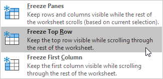
To freeze the top row, execute the following steps.
1. On the View tab, click Freeze Panes, Freeze Top Row.

2. Scroll down to the rest of the worksheet.
Result. Excel automatically adds a black horizontal line to indicate that the top row is frozen.

Note: to keep the first column visible while scrolling through the right of the worksheet, click Freeze First Column.
To unlock all rows and columns, execute the following steps.
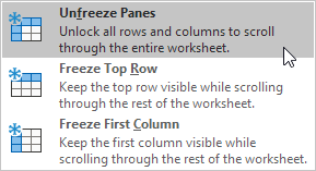
1. On the View tab, click Freeze Panes, Unfreeze Panes.

To freeze panes, execute the following steps.
1. Select row 3.
2. On the View tab, click Freeze Panes, Freeze Panes.

3. Scroll down to the rest of the worksheet.
Result. All rows above row 3 are frozen.

Note: to keep columns visible while scrolling to the right of the worksheet, select a column and click Freeze panes.
4. Select cell C3 (unfreeze panes first).
5. On the View tab, click Freeze Panes, Freeze Panes.
Result. The region above row 3 and to the left of column C is frozen.


Answer is in your question itself....select the row/coloumn and select Freeze option from the menu. it should work.
Uses : simply comparing the standard values with other row/coloumns corresponding/related data
-- for the purpose of heading, etc. My 2 cents. Thanks.

Thanks for the invitation; a Smart Question indeed.
I prefer awaiting response from other Colleagues.

Ever find yourself in the middle of a long spreadsheet, having forgotten which column is which and needing to scroll all the way back to the table headings to make sense of what you’re looking at? Not exactly a fun way to spend your time. Nor is it the most efficient.
That’s why you’ll be glad to know there is a way to keep all of the identifying information in view as you scroll down rows and rows of data.
Freeze the first row
The most common need that you will experience with Excel is, no doubt, to keep your column headings in place. So that is where we’ll start. It’s a simple operation and really just involves knowing where to look.
Assuming you’ve got your workbook open to the spreadsheet you need, follow these steps.
1. Click on the View tab from the main menu.
2. From the View Ribbon, select Freeze Panes, which will bring up a dropdown menu.
3. Select the Freeze top row option from the dropdown menu.
Remember that, even though it is the column headings you want to stay in place, it is the top row you want frozen, because this is where that information will be placed. You’ll know that the process has been successful if a black border appears under the top row. Then to confirm, simply scroll down the spreadsheet, and your column headings should remain in place.
Freeze the first column
In some cases, you will be looking at a lot of records that, for whatever reason, require you to scroll horizontally across the spreadsheet, rather than vertically. If you find yourself with in this situation, you can use the freeze pain function on your initial column, rather than the top row, so that you can keep the row labels in view.
Here is the procedure to follow:
1. Click on the View tab to bring up the View ribbon.
2. Select Freeze Panes, which will bring you the dropdown menu for the feature.
3. Select Freeze First Column, since this column will contain your row labels.
You should see a black border along the right side of the first column. You can then scroll horizontally to confirm that the procedure was successful.
Freeze columns and rows
Once in a while, you come across that spreadsheet that is just chocking full of data. Not only does it have a multitude of record entries for its columns, but it also has a seemingly endless list of data entries filling up the rows. In this case, you will want to freeze panes for both the rows and the columns to make it easier on yourself as you navigate the sheet. Here’s what you’ll do:
1. Select the first cell inside the table that is not a row or column label. For instance, if your columns are listed across row 1 and your rows are labeled down column A, you will want to select column B2.
2. Cick on the View tab from the main menu.
3. Click on Freeze Panes to bring up the drop-down menu.
4. Select the option labeled Freeze Panes.
This time, you should see a black border both under your column headings and to the right of your row labels. You can test out whether you were successful by scrolling both horizontally and vertically. Your first row and your first column should both remain in place as you do.
Unfreeze
Sometimes, you may not want to keep the Freeze Panes feature turned on after you have finished with the spreadsheet. And, as you would hope, Microsoft has planned for that. Also, as you might have guessed, you will be using roughly the same procedure, with a different option from the dropdown menu. Here are the steps for unfreezing the panes:
1. Click on the View tab
2. Select the Freeze panes option
3. From the drop-down menu, select unfreeze panes.
The black borders will have disappeared and column/row labels will no longer follow along with you as you scroll within the spreadsheet.
I hope my answer is helpful and Thanks for the Invitation Danish Shafiq! Good Job!
Freeze panes to lock specific rows or columns. On the worksheet, do one of the following: To lock rows, select the row below the row or rows that you want to keep visible when you scroll.

thanks for the invitation and agree with the answers of experts.

Freeze pane is mostly use for the large Excel sheet where the rows & columns are more than the screen size. To view certain fixed area of the Excel sheet commonly used freeze pane.
keep it up and all user correctly answer this question.

Whenever you're working with a lot of data, it can be difficult to compare information in your workbook. Fortunately, Excel includes several tools that make it easier to view content from different parts of your workbook at the same time, such as the ability to freeze panes and split your worksheet.
To freeze rows:
You may want to see certain rows or columns all the time in your worksheet, especially header cells. By freezing rows or columns in place, you'll be able to scroll through your content while continuing to view the frozen cells.
1. Select the row below the row(s) you want to freeze.
2. Click the View tab on the Ribbon.
3. Select the Freeze Panes command, and then choose Freeze Panes from the drop-down menu.
4. The rows will be frozen in place, as indicated by the gray line. You can scroll down the worksheet while continuing to view the frozen rows at the top.
To freeze columns:
1. Select the column to the right of the column(s) you want to freeze.
2. Click the View tab on the Ribbon.
3. Select the Freeze Panes command, and then choose Freeze Panes from the drop-down menu.
4. The column will be frozen in place, as indicated by the gray line. You can scroll across the worksheet while continuing to view the frozen column on the left.
To unfreeze rows or columns, click the Freeze Panes command, then select Unfreeze Panes from the drop-down menu.
If you only need to freeze the top row (row 1) or first column (column A) in the worksheet, you can simply select Freeze Top Row or Freeze First Column from the drop-down menu.


Do you need help in adding the right keywords to your CV? Let our CV writing experts help you.